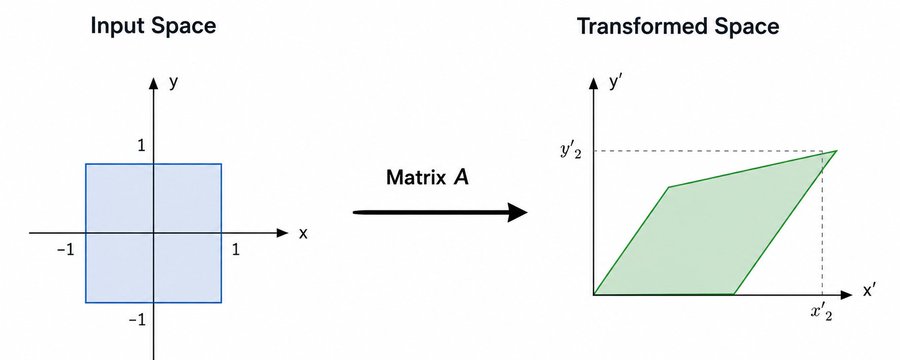
If you have spent any time around machine learning, you have probably seen this formula:
A = UΣVᵀ
At first, it looks like someone took one matrix and made the problem worse by replacing it with three matrices. But SVD is not trying to make the matrix more complicated. It is trying to expose what the matrix was doing all along.
1. The problem with how SVD is usually introduced
Most explanations start with the formula too early:
A = UΣVᵀ
That is technically correct, but it does not answer the real question: why should such a factorization exist at all?
As an engineer, the formula feels backwards. You are shown the final decomposition before you understand the transformation it is decomposing.
A better way to approach SVD is to forget the formula for a moment and ask: what does a matrix actually do to space? That question makes the whole thing much less mysterious.
2. A matrix is not just a table of numbers
A 2 × 2 matrix like A = [a b; c d] is not just four values arranged neatly. It is a function—usually a linear function—that moves vectors.
Give it a vector x, and it produces a new vector Ax. If you apply it to every point in the plane, the whole plane moves.
The important part:
- Lines remain lines.
- The origin stays fixed.
- Parallel lines remain parallel.
- Distances, angles, areas, and directions can change.
So a matrix is better imagined as a machine that transforms space. If you apply a matrix to a square, it may rotate, stretch, shear, or flip it.
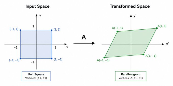
This is where SVD enters. It asks: can this complicated-looking transformation be understood as a few simple transformations? The answer is yes.
3. The circle experiment
Instead of watching what a matrix does to a square, watch what it does to a circle.
Start with the unit circle:
x₁² + x₂² = 1
Every point on this circle has the same length: 1.
Now apply the matrix A to every point on the circle. In general, the circle becomes an ellipse.
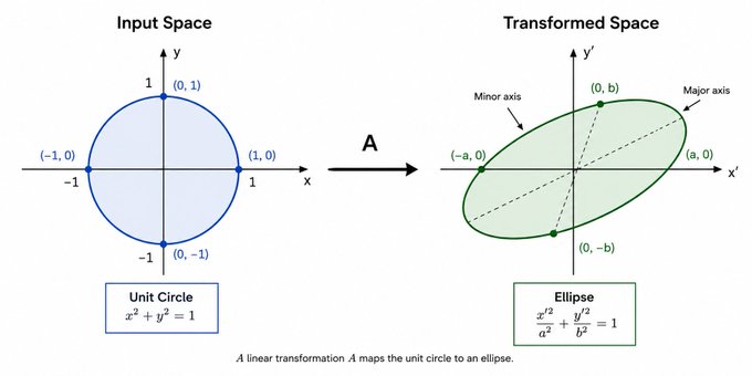
This picture is the core intuition behind SVD. The original circle treats all directions equally; the ellipse does not.
Some directions are stretched a lot. Some directions are stretched only a little.
The longest axis of the ellipse tells us: this was the direction of maximum stretching. The shortest axis tells us: this was the direction of minimum stretching.
If you know these axes, you know the important behavior of the matrix. That is what SVD extracts.
4. The three things SVD finds
SVD looks at a matrix and finds three kinds of information:
- Input directions. These are the special directions before the matrix acts. They are called the right singular vectors.
- Stretch amounts. These tell us how much each special direction gets stretched. They are the singular values.
- Output directions. These are where the special directions land after transformation. They are called the left singular vectors.
In 2D, this idea can be written as:
Av₁ = σ₁u₁
Av₂ = σ₂u₂
Meaning:
vᵢis the input direction.σᵢis the stretch factor.uᵢis the output direction.
This is already the meaning of SVD. The full matrix formula is just a compact way to write it.
5. Why are eigenvectors not enough?
A natural question is: why not just use eigenvectors?
Eigenvectors describe directions that stay on the same line:
Av = λv
This is useful, but it is also restrictive.
A pure 90-degree rotation has no real eigenvector in 2D, because every vector is rotated away from its original line. But the rotation is not mysterious—it simply preserves length and changes direction.
SVD handles this cleanly because it does not require directions to stay on the same line.
Eigenvectors ask: which directions remain aligned with themselves? SVD asks: which directions get stretched, and by how much?
That second question is more useful for understanding general transformations, especially rectangular and high-dimensional matrices.
6. The one equation that reveals the hidden directions
Suppose x is a unit vector. After applying A, its new length is ‖Ax‖.
To study stretching, look at the squared length:
‖Ax‖² = (Ax)ᵀ(Ax) = xᵀAᵀAx
The stretching behavior of A is encoded inside AᵀA.
Why does this help? Because AᵀA is symmetric, and symmetric matrices have clean perpendicular eigenvectors. Those eigenvectors become the input directions of SVD.
This is the small piece of math that makes the geometry precise.
7. A tiny SVD code snippet
Before jumping into why this matters for LLMs, here is a tiny implementation of SVD for a 2 × 2 matrix. The goal is not to replace numpy.linalg.svd, but to see the geometry turn into code.
import math
import numpy as np


def normalize(v, tol=1e-12):
    norm = math.sqrt(float(np.dot(v, v)))
    if norm < tol:
        raise ValueError("Cannot normalize a near-zero vector.")
    return v / norm


def svd_2x2(A, tol=1e-12):
    A = np.asarray(A, dtype=float)

    if A.shape != (2, 2):
        raise ValueError("This demo only handles 2 by 2 matrices.")

    a, b = A[0, 0], A[0, 1]
    c, d = A[1, 0], A[1, 1]

    # Build A^T A. This matrix reveals the hidden stretch directions.
    p = a * a + c * c
    q = a * b + c * d
    r = b * b + d * d
    B = np.array([[p, q], [q, r]], dtype=float)

    # One Jacobi rotation diagonalizes a symmetric 2 by 2 matrix.
    theta = 0.5 * math.atan2(2.0 * q, p - r)
    cos_t = math.cos(theta)
    sin_t = math.sin(theta)
    V = np.array([[cos_t, -sin_t], [sin_t, cos_t]], dtype=float)

    D = V.T @ B @ V
    lambdas = np.clip(np.diag(D), 0.0, None)

    # Sort singular values from largest to smallest.
    order = np.argsort(lambdas)[::-1]
    lambdas = lambdas[order]
    V = V[:, order]
    sigmas = np.sqrt(lambdas)
    Sigma = np.diag(sigmas)

    # Recover output directions using u_i = A v_i / sigma_i.
    u_columns = []
    for i, sigma in enumerate(sigmas):
        if sigma > tol:
            u_columns.append(normalize(A @ V[:, i]))

    if len(u_columns) == 0:
        U = np.eye(2)
    elif len(u_columns) == 1:
        u1 = u_columns[0]
        u2 = np.array([-u1[1], u1[0]])
        U = np.column_stack([u1, u2])
    else:
        u1, u2 = u_columns
        u2 = normalize(u2 - np.dot(u1, u2) * u1)
        U = np.column_stack([u1, u2])

    return U, Sigma, V.T


A = np.array([[3.0, 1.0], [0.0, 2.0]])
U, Sigma, Vt = svd_2x2(A)

print(U)
print(Sigma)
print(Vt)
print(U @ Sigma @ Vt)
8. Why low-rank approximation falls out naturally
SVD can also be written as a sum of simpler pieces:
A = σ₁u₁v₁ᵀ + σ₂u₂v₂ᵀ + …
Each term represents one direction of behavior. The singular value σᵢ tells you how important that direction is.
If the singular values look like this—100, 42, 11, 2, 0.1, 0.01—most of the matrix’s useful behavior is concentrated in the first few directions. So instead of keeping the full matrix, keep only the top k directions:
Aₖ = UₖΣₖVₖᵀ
This is low-rank approximation.
The intuition is simple: a large transformation may be mostly explained by a small number of important directions.
This is why SVD appears in compression, PCA, recommendation systems, denoising, and representation learning.
9. Why this matters for LLMs
Modern language models are full of huge matrices. There are matrices for:
- Token embeddings
- Query projections
- Key projections
- Value projections
- Feed-forward layers
- Output projections
A transformer may look complicated, but a huge amount of its work is matrix multiplication. SVD is not usually computed during every forward pass of an LLM; that is not the point.
The important idea is this: big matrices often contain structure that is much smaller than the matrix itself.
Once you believe that, many modern techniques start to make more sense:
- Low-rank approximation
- Model compression
- Efficient fine-tuning
- Adapter methods
- LoRA
SVD gives the mental model behind these ideas.
10. LoRA through the SVD lens
Suppose a model has a large weight matrix W.
Full fine-tuning updates the whole matrix:
W ← W + ΔW
But ΔW can be huge. LoRA makes a different bet: the useful task-specific update may live in a much smaller subspace. So instead of learning a full update matrix, LoRA learns two smaller matrices:
ΔW = BA
The product BA is low-rank. This is not the same as computing the SVD of W, but the intuition is related:
- SVD says a matrix can often be approximated using fewer important directions.
- LoRA says a fine-tuning update can often be learned using fewer important directions.
We may not need the full matrix to capture the useful behavior.
This exploration was inspired by Deep-ML Problem 12.